Image blind denoising based on Gibbs-Diffusion

Tutorial Introduction

GDiff stands for Gibbs-Diffusion, a Bayesian blind denoising method that solves the problem of posterior sampling of signal and noise parameters. It relies on a Gibbs sampler that alternates sampling steps with a pre-trained diffusion model (defining the signal prior) and a Hamiltonian Monte Carlo sampler. The paper introduces its applications in natural image denoising and cosmology (cosmic microwave background analysis). The paper results are "Listening to the Noise: Blind Denoising with Gibbs Diffusion"

The official document only gives the test method, which is to pass in a clear original image, superimpose noise, and then perform non-blind denoising and blind denoising comparison.

Effect Demonstration

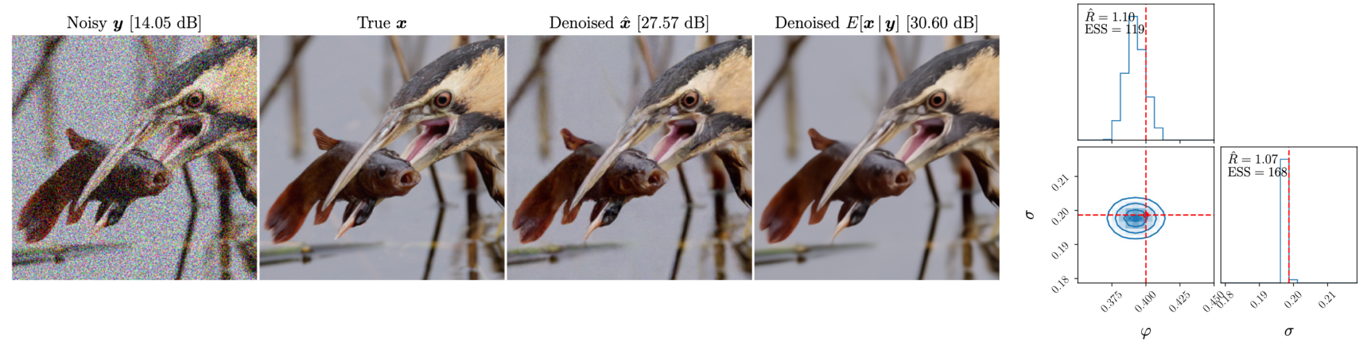
In the official effect demonstration, a clear original image is input, noise with certain parameters is superimposed on it, and then blind denoising is performed.

The following figures are from left to right: the image after superimposing noise, the original image, the blind denoising effect, and the denoised posterior mean

Introduction to blind denoising and non-blind denoising

Blind denoising and non-blind denoising are two denoising methods in image processing and signal processing. The main difference between them lies in the degree of prediction of noise information.

Blind Denoising

Definition: Blind denoising refers to denoising without knowing the noise characteristics or noise model. This method does not rely on prior knowledge of noise, but denoises through the information of the image or signal itself.

Features:

• Noise model independent: no knowledge of the noise type, distribution or intensity is required.
• Strong adaptability: can be applied to various types of noise and signal environments.
• High complexity: Since there is no help from the noise model, blind denoising usually requires more complex algorithms and more computing resources.

Non-blind denoising

Definition: Non-blind denoising refers to denoising when the noise characteristics or noise model are known. This method uses prior knowledge of noise to optimize the denoising process.

Features:

• Dependence on noise model: It requires prior knowledge of the type, distribution, and intensity of noise.
• Better effect: When the noise model is known, it can be optimized for specific noise types to achieve better denoising effect.
• Limited scope of application: Different models and parameters are required for different types of noise, and the scope of application is narrower than blind denoising.

How to run the tutorial

This tutorial is divided into two parts. The first part is "Blind Denoising of Blurred Images", which can be run in the start.ipynb file (this file). Here, you can pass in a blurred image with noise for blind denoising. The second part is "Clear Image Superimposed Noise and Denoising", which is run in the test.ipynb file. This is a simplification of the official document and can be used to pass in clear images with superimposed noise to compare the difference between the blind denoising model and the non-blind denoising model.

If you need to use custom images, just upload the images and modify the path of the images you want to process, and run them one by one. (The image name must be in English)

Part 1: Blind Denoising of Blurred Images (start.ipynb)

Import required packages

import sys, time
import torch
import numpy as np
import matplotlib.pyplot as plt
import corner
import arviz as az
from PIL import Image

sys.path.append('..')

from gdiff.data import ImageDataset, get_colored_noise_2d
from gdiff.model import load_model
import gdiff.hmc_utils as iut
from gdiff.utils import ssim, psnr, plot_power_spectrum, plot_list_of_images

plt.rcParams.update(
{
'text.usetex': False,
    'font.family': 'stixgeneral',
'mathtext.fontset': 'stix',
}
)

Image reading and preprocessing functions, usage is from the official document data.py

#图片读取与预处理，方法来自官方文档 data.py
def readimg(filename):
    from torchvision import transforms
    img=Image.open(filename)
    trans = transforms.Compose([transforms.Resize(256),
                                            transforms.CenterCrop(256),
                                            transforms.RandomHorizontalFlip(),
                                            transforms.ToTensor()])
    img=trans(img)
    return img

The following is the official method for reading datasets, which is not used in this document. Users can put their own datasets in their folders and make some minor modifications to achieve batch processing (only a few folder names can be selected, in the data folder)

#
# PARAMETERS 官方数据读取与噪声参数，模型选择
#

# Dataset and sample 读取官方数据集
dataset_name = "CBSD68" # Choices among "imagenet_train", "imagenet_val", "CBSD68", "McMaster", "Kodak24"
dataset = ImageDataset(dataset_name, data_dir='./data')
sample_id = 0 # np.random.randint(len(dataset))

# Noise 准备叠在在清晰图片上的噪声
phi_true = -0.4     # Spectral index -> between -1 and 1 (\varphi in the paper)
sigma_true = 0.1    # Noise level

# Device 
device = torch.device('cuda' if torch.cuda.is_available() else 'cpu')

# Model 选择模型，有 5000 与 10000 步迭代模型可选
diffusion_steps = 5000 # Number of diffusion steps: 5000 or 10000
model = load_model(diffusion_steps=diffusion_steps,
                   device=device,
                   root_dir='./model_checkpoints')
model.eval()

# Inference 
num_chains = 4      # Number of HMC chains
n_it_gibbs = 50     # Number of Gibbs iterations after burn-in
n_it_burnin = 25    # Number of burn-in iterations

Next, read the image that needs to be denoised. For example, the image used in this tutorial is '3_noisy.png' in the home directory. In img=readimg('3_noisy.png'), simply change the path to '3_noisy.png'.

In the case of A6000 with a single card, it takes several minutes to process a single image.

#
# DENOISING 在此处读入的图片为高噪声图，在此处进行降噪处理
#
 
# 读取自己的高噪声图片，用于去噪
img=readimg('3_noisy.png')
x = img.to(device).unsqueeze(0)

# Our DDPM has discrete timestepping -> we get the time step closest to the chosen noise level
sigma_true_timestep, sigma_true = model.get_closest_timestep(torch.tensor([sigma_true]), ret_sigma=True)
alpha_bar_t = model.alpha_bar_t[sigma_true_timestep.cpu()].reshape(-1, 1, 1, 1).to(device)
print(f"Time step corresponding to noise level {sigma_true.item():.3f}: {sigma_true_timestep.item()}")
yt = torch.sqrt(alpha_bar_t) * x # Noisy image normalized for the diffusion model 归一化图像

# Non-blind denoising (for reference) 非盲去噪 即已知噪声参数的情况下去噪

print("Denoising in non-blind setting...")
t0 = time.time()
x_hat_nonblind = model.denoise_samples_batch_time(yt,
                                                  sigma_true_timestep.unsqueeze(0),
                                                  phi_ps=phi_true)
t1 = time.time()
print(f"Non-blind denoising took {t1-t0:.2f} seconds")

# Blind denoising with GDiff 基于 GDiff 的盲去噪
print("Denoising in blind setting (GDiff)...")
t0 = time.time()
phi_hat_blind, x_hat_blind = model.blind_denoising(x, yt,
                                                   num_chains_per_sample=num_chains,
                                                   n_it_gibbs=n_it_gibbs,
                                                   n_it_burnin=n_it_burnin)
t1 = time.time()
print(f"Blind denoising took {t1-t0:.2f} seconds")

# Denoised posterior mean estimate 去噪的后验均值估计
x_hat_blind_pmean = x_hat_blind[:, n_it_burnin:].mean(dim=(0, 1))

Time step corresponding to noise level 0.100: 134 Denoising in non-blind setting... Non-blind denoising took 4.48 seconds Denoising in blind setting (GDiff)...

  0%| | 0/75 [00:00

Adapting step size using 300 iterations Step size fixed to : tensor([0.0179, 0.0181, 0.0179, 0.0194], device='cuda:0')

100%|██████████| 75/75 [08:52<00:00, 7.10s/it]

Blind denoising took 532.30 seconds

#
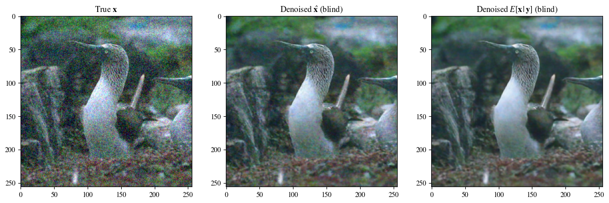
# Plot of a reconstruction 展示结果 顺序为：原始图片 非盲去噪 盲去噪 去噪的后验均值
#

data = [x[0],
        x_hat_blind[0, -1],
        x_hat_blind_pmean]
data = [d.to(device) for d in data]
labels_base = [r"True $\mathbf{x}$",
          r"Denoised $\hat{\mathbf{x}}$ (blind)",
          r"Denoised $E[\mathbf{x}\,|\,\mathbf{y}]$ (blind)"]

labels = [labels_base[0] ,
          labels_base[1] ,
          labels_base[2] ]
plot_list_of_images(data, labels)
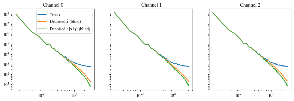
plot_power_spectrum(data, labels_base, figsize=(12, 3.5))

Clipping input data to the valid range for imshow with RGB data ([0..1] for floats or [0..255] for integers).